半導体材料抵抗率の高精度な測定方法(High-precision semiconductor resistivity measurement)
To measure the resistivity of semiconductors, the four-point probe method is a well used technique.
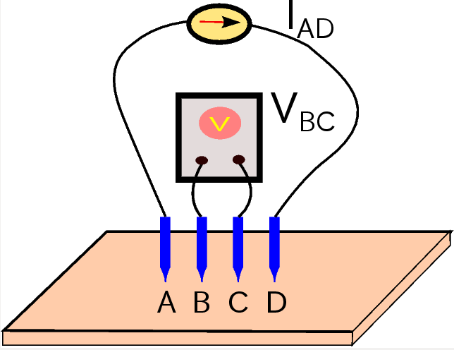
As shown in above Figure, in this method, four probes $A$, $B$, $C$ and $D$ with equal intervals are aligned on the surface of a semiconductor object and a constant current $I_{AD}$ is imposed on $(A,D)$ pair and the floating potential $V_{BC}$ between $(B,C)$ pair is measured. Suppose the semiconductor object has a constant resistivity $\rho$. The resistivity of the semiconductor object is expected to be calculate by using $V_{BC}$ and $I_{AD}$, $$ \rho = F(V_{BC}/I_{AD}), $$ where the function $F$ is a function to be determined and is called by geometrical correction factor. Such a factor is dependent on the geometric shape of the object, the position of the probe and the distance among the points $A$, $B$, $C$ and $D$. The objective of this research is to give a verified evaluation of this factor $F$.

As shown in above Figure, in this method, four probes $A$, $B$, $C$ and $D$ with equal intervals are aligned on the surface of a semiconductor object and a constant current $I_{AD}$ is imposed on $(A,D)$ pair and the floating potential $V_{BC}$ between $(B,C)$ pair is measured. Suppose the semiconductor object has a constant resistivity $\rho$. The resistivity of the semiconductor object is expected to be calculate by using $V_{BC}$ and $I_{AD}$, $$ \rho = F(V_{BC}/I_{AD}), $$ where the function $F$ is a function to be determined and is called by geometrical correction factor. Such a factor is dependent on the geometric shape of the object, the position of the probe and the distance among the points $A$, $B$, $C$ and $D$. The objective of this research is to give a verified evaluation of this factor $F$.
Mathematical model
Let $\Omega$ be the domain of the semiconductor object.
Given the positions for probes $A$ and $D$, denoted by ${\bf r}_A$ and ${\bf r}_D$ respectively,
the potential $\Phi(r)$ inside the semiconductor object is the solution of the
following Poisson's equation in $R^3$.
\begin{equation}
\label{basic-model}
\Delta \Phi({\bf r}) = 2 \rho I_{AD} \left( \delta({\bf r}-{\bf r}_D) - \delta({\bf r}-{\bf r}_A)\right) \mbox{ in }\Omega; \quad \frac{\partial \Phi}{\partial n}=0 \mbox{ on }\partial \Omega , \quad\quad\quad\quad (1)
\end{equation}
where $\delta$ is the Dirac delta function in $R^3$.
Define $Q({\bf r}) := \Phi({\bf r})/(\rho\cdot I_{AD})$. Theoretically, the value of $Q({\bf r})$ can be uniquely determined by solving the equation (1). In practical measurement, the following value is known from measured $V_{BC}$ and $I_{AD}$. $$ \tilde{\rho}: = \frac{V_{BC}}{I_{AD}}. $$ Since $V_{BC} =\Phi({\bf r}_C) - \Phi({\bf r}_B)$, we have $$ \tilde{\rho} = \rho \cdot \left( { Q({\bf r}_C) - Q({\bf r}_B) } \right). $$ Thus the resistivity $\rho$ can be calculated by $$ \rho = \frac{ \tilde{\rho}}{ Q({\bf r}_C) - Q({\bf r}_B) } = F_c \cdot \tilde{\rho}\quad (F_c:= \frac{1}{ Q({\bf r}_C) - Q({\bf r}_B) }). $$ Here, $F_c$, as the geometric correction factor, is to be evaluated by solving (1).
In this research, we will develop an efficent method to sovle the above equation to calcualte $F$ with high-precision.
Define $Q({\bf r}) := \Phi({\bf r})/(\rho\cdot I_{AD})$. Theoretically, the value of $Q({\bf r})$ can be uniquely determined by solving the equation (1). In practical measurement, the following value is known from measured $V_{BC}$ and $I_{AD}$. $$ \tilde{\rho}: = \frac{V_{BC}}{I_{AD}}. $$ Since $V_{BC} =\Phi({\bf r}_C) - \Phi({\bf r}_B)$, we have $$ \tilde{\rho} = \rho \cdot \left( { Q({\bf r}_C) - Q({\bf r}_B) } \right). $$ Thus the resistivity $\rho$ can be calculated by $$ \rho = \frac{ \tilde{\rho}}{ Q({\bf r}_C) - Q({\bf r}_B) } = F_c \cdot \tilde{\rho}\quad (F_c:= \frac{1}{ Q({\bf r}_C) - Q({\bf r}_B) }). $$ Here, $F_c$, as the geometric correction factor, is to be evaluated by solving (1).